Notes on developing an IIR filter using MATLAB's filter design tool
© Harry Broeders - Hogeschool Rotterdam.
 This page is meant for student of the minor Embedded
Systems at Rotterdam University or anyone who wants to develop IIR filters
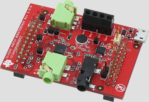
using MATLAB's filter design tool. To implement and test the filters the CC3200AUDBOOST Audio
BoosterPack (shown on the right) and the CC3220S LaunchPad boards
from Texas Instruments are used. An introduction which describes how to install
the proper software to experiment with these boards can be found here: Introduction to using the CC3200AUDBOOST and CC3220S
LAUNCHXL. The CC3220S Launchpad contains the CC3220S System on Chip (SoC)
which contains an user application dedicated ARM® Cortex®-M4 MCU. Because the
Cortex®-M4 has no hardware support for floating point calculations, our intent
is to develop a filter using fixed-point arithmetic. Developing a FIR filter
using fixed-point arithmetic was relatively straightforward but developing an
IIR filter using fixed-point arithmetic proved to be more difficult than
expected. This page will describe the problems found and their solutions.
This page is meant for student of the minor Embedded
Systems at Rotterdam University or anyone who wants to develop IIR filters
using MATLAB's filter design tool. To implement and test the filters the CC3200AUDBOOST Audio
BoosterPack (shown on the right) and the CC3220S LaunchPad boards
from Texas Instruments are used. An introduction which describes how to install
the proper software to experiment with these boards can be found here: Introduction to using the CC3200AUDBOOST and CC3220S
LAUNCHXL. The CC3220S Launchpad contains the CC3220S System on Chip (SoC)
which contains an user application dedicated ARM® Cortex®-M4 MCU. Because the
Cortex®-M4 has no hardware support for floating point calculations, our intent
is to develop a filter using fixed-point arithmetic. Developing a FIR filter
using fixed-point arithmetic was relatively straightforward but developing an
IIR filter using fixed-point arithmetic proved to be more difficult than
expected. This page will describe the problems found and their solutions.
MATLAB's filter design tool
MATLAB offers a filter design tool. This tool was named fdatool (filter
design and analysis tool) before version 2016 of MATLAB and is renamed
filterDesigner since version 2016. More information about this tool can be
found here:
Developing an IIR filter using a floating-point implementation
We first developed an IIR filter using 32 bit (single-precision)
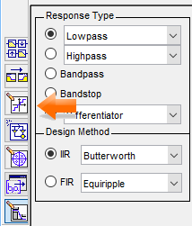
floating-point arithmetic. A low-pass Butterworth filter of order 2 with a
sample frequency of 8 KHz and a cutoff frequency of 1 KHz was designed by using
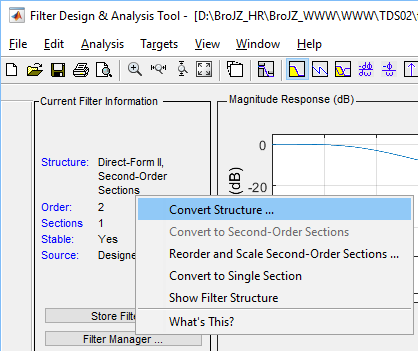
MATLAB's filter designer. The default implementation used by the filter
designer tool is a direct-form II with second-order sections. This is converted
into a direct-form I by right clicking on the structure information in the
current filter information pane and choosing Convert
Structure....
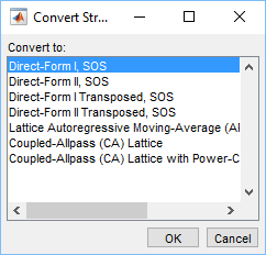
Then choose Direct-Form I, SOS.
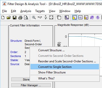
Now convert the implementation from SOS (Second-Order Sections) into a
single section by right clicking on the structure information in the current
filter information pane again and choosing Convert to
Single Section.
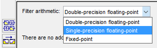
The default implementation used double-precision (64 bits) floating-point
arithmetic but we want to use single-precision (32 bits) arithmetic. This can
be changed by clicking the Set quantization parameters button on the left side
of the filter design tool.
Choose Single-precision floating-point from
the pull-down menu.
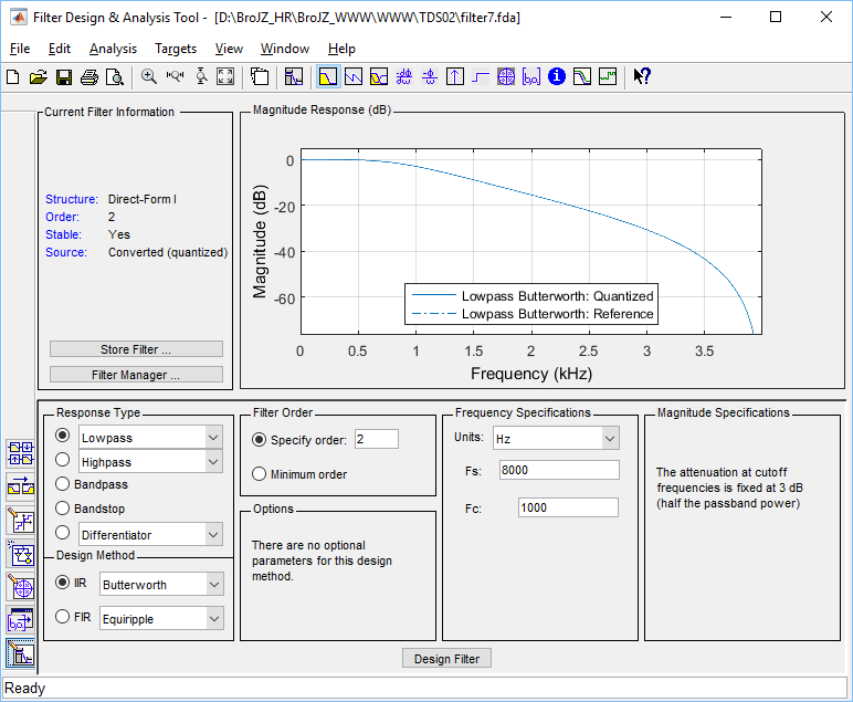
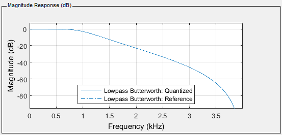
The resulting filter design is shown below. The .fda file which can be
opened in MATLAB can be found here: filter7.fda.
The filter coefficients can be exported to a header file by using the menu
option Targets, Generate C header ...:
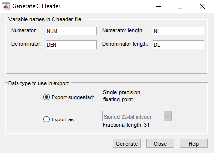
The generated header file can be found here: filter7.h.
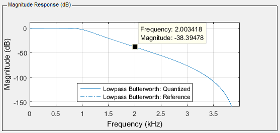
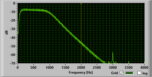
When we implement this filter using float variables and measure
the magnitude response using the soundcard oscilloscope program which can be
found at https://www.zeitnitz.eu/scms/scope_en,
we get the following result.
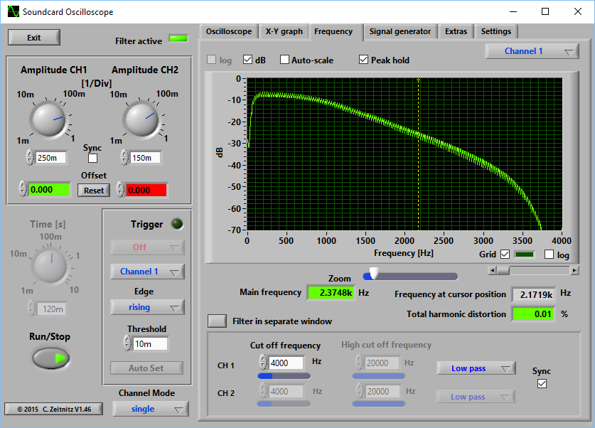
The filter is working as expected.
When we try to increase the order to 3 the filter does not work correctly
anymore because the implementation is not fast enough (the calculation of the
next output sample is not finished when the next input sample arrives). The
required output and the actual output are shown below.
So if we want to implement higher order IIR filters using the TMS320C5505 we
have to use fixed-point arithmetic.
Developing an IIR filter using a fixed-point implementation
Moving to a fixed-point implementation of the second order IIR filter seems
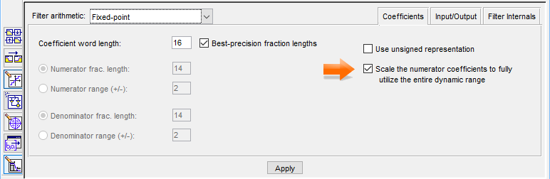
trivial but we encountered some problems. By clicking the Set quantization
parameters button on the left side of the filter design tool we changed the
filter arithmetic to Fixed-point and checked the
option Scale the numerator coefficients to fully
utilize the entire dynamic range. We choose to check this option because
it seems logical to do so (who doesn't want to utilize the entire dynamic
range?).
The .fda file which can be opened in MATLAB can be found here: filter9.fda. The generated header file can be found
here: filter9.h.
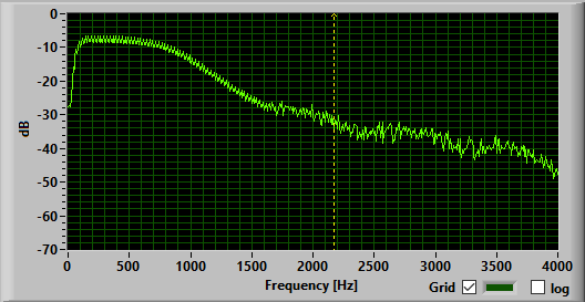
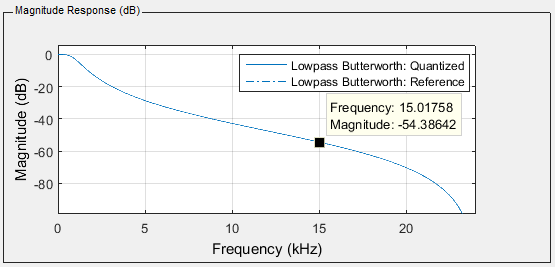
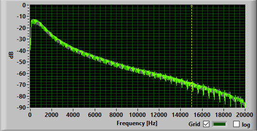
This filter does not work as expected. The required output and the actual
output are shown below.
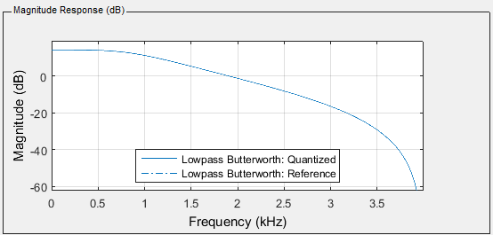
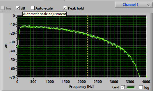
At first glance it seems almost correct but when we look closer we see that
it is clearly wrong. E.g. the attenuation of the signal at 2 KHz should be
about 16 dB but actually is only about 6 dB.
We now compare the single-precision floating-point coefficients (found in filter7.h) with the fixed-point coefficients (found in filter9.h).
Here are the coefficients in single-precision floating-point notation
without scaling (found in filter7.h):
const int NL = 3;
const real32_T NUM[3] = {    0.09763107449,    0.195262149,  0.09763107449};
const int DL = 3;
const real32_T DEN[3] = {                1,  -0.9428090453,   0.3333333433};
Here are the coefficients in fixed-point notation s16.14
with scaling (found in filter9.h):
const int NL = 3;
const int16_T NUM[3] = {     8192,  16384,   8192};
const int DL = 3;
const int16_T DEN[3] = {    16384, -15447,   5461};
We can convert these fixed-point s16.14 numbers back into floating-point
notation by dividing them by 214. The coefficients in
single-precision floating-point notation with scaling are:
const int NL = 3;
const real32_T NUM[3] = {              0.5,            1.0,            0.5};
const int DL = 3;
const real32_T DEN[3] = {                1,  -0.9428100586,   0.3333129882};
We can observe now that MATLAB has scaled the numerator coefficients by
1/0.195262149. The denumerator coefficients on the other hand are not scaled the at all! This is not correct and therefore
the option Scale the numerator coefficients to fully
utilize the entire dynamic range must be unchecked!

The .fda file which can be opened in MATLAB can be found here: filter10.fda. The generated header file can be found
here: filter10.h.
The most important parts of this header file is shown below:
/*
 * Discrete-Time IIR Filter (real)
 * -------------------------------
 * Filter Structure    : Direct-Form I
 * Numerator Length    : 3
 * Denominator Length  : 3
 * Stable              : Yes
 * Linear Phase        : No
 * Arithmetic          : fixed
 * Numerator           : s16,17 -> [-2.500000e-01 2.500000e-01)
 * Denominator         : s16,14 -> [-2 2)
 * Input               : s16,15 -> [-1 1)
 * Output              : s16,15 -> [-1 1)
 * Numerator Prod      : s32,32 -> [-5.000000e-01 5.000000e-01)
 * Denominator Prod    : s32,29 -> [-4 4)
 * Numerator Accum     : s34,32 -> [-2 2)
 * Denominator Accum   : s34,29 -> [-16 16)
 * Round Mode          : convergent
 * Overflow Mode       : wrap
 */

const int NL = 3;
const int16_T NUM[3] = {
     1600,   3199,   1600
};
const int DL = 3;
const int16_T DEN[3] = {
    16384, -15447,   5461
};
The comments suggest that the Numerator coefficients are coded in s16.17
fixed-point and that the Denumerator coefficients are coded in s16.14
fixed-point. Therefore the Numerator Accumulation must be shifted three bits to
the right before the Denumerator Accumulation can be subtracted (the binary
points should be properly aligned before an addition or subtraction can be
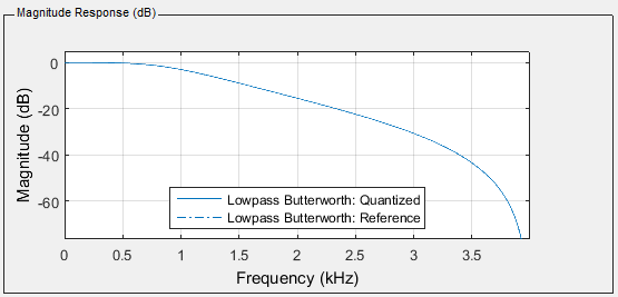
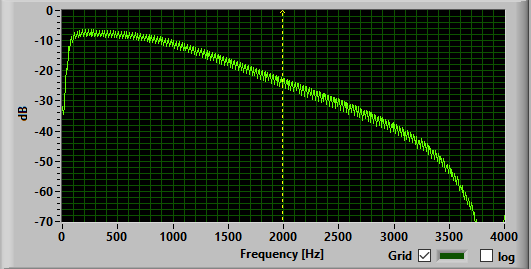
performed).Implementing this filter accordingly does not result in the correct
behavior!
If we convert the generated coefficients found in filter10.h back to floating-point we discover that
all coefficients are in s16.14
notation. Therefore the Numerator Accumulation must
not be shifted before the Denumerator
Accumulation is subtracted! Implementing this results in filter which works as
expected. The required output and the actual output are shown below.
It is now possible to implement higher order filters. E.g. the required
output and the actual output of a fifth order filter are given below. The .fda
file which can be opened in MATLAB can be found here: filter11.fda. The generated header file can be found
here: filter11.h.
Using fixed-point arithmetic it is also possible to use a higher sample
frequency. For example, the required output and the actual output of a low-pass
Butterworth filter of order 2 with a sample frequency of 48 KHz and a cutoff
frequency of 1 KHz are given below. The .fda file which can be opened in MATLAB
can be found here: filter12.fda. The generated
header file can be found here: filter12.h.
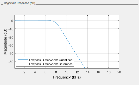
Finally, (just to show off) the required output and the actual output of a
low-pass Butterworth filter of order 9 with a sample frequency of 48 KHz and a
cutoff frequency of 8 KHz are given below. The .fda file which can be opened in
MATLAB can be found here: filter15.fda. The
generated header file can be found here: filter15.h.

To be fair, I had to optimize my code before this one was working correctly
;-).